cleaning the dataset
Statistical testing
library(corrplot)## corrplot 0.84 loaded#test to see if there is a relationship between
#sex and income
test<-chisq.test(table(df3$sex, df3$income))
test##
## Pearson's Chi-squared test
##
## data: table(df3$sex, df3$income)
## X-squared = 42.441, df = 9, p-value = 2.729e-06table(df3$sex, df3$income)##
## <10 10-20 20-30 30-40 40-50 50-75 75-100 100-150 >150 NA
## Male 99 138 132 135 100 211 149 126 98 138
## Female 145 176 185 171 149 203 149 134 73 256The p-value = .000002729 to test for independence gender and “income” we found we would reject independence and assumed that income is dependent on gender. With this we can assume a gender wage gap for workers in our study.
corrplot(test$residuals, is.corr = F)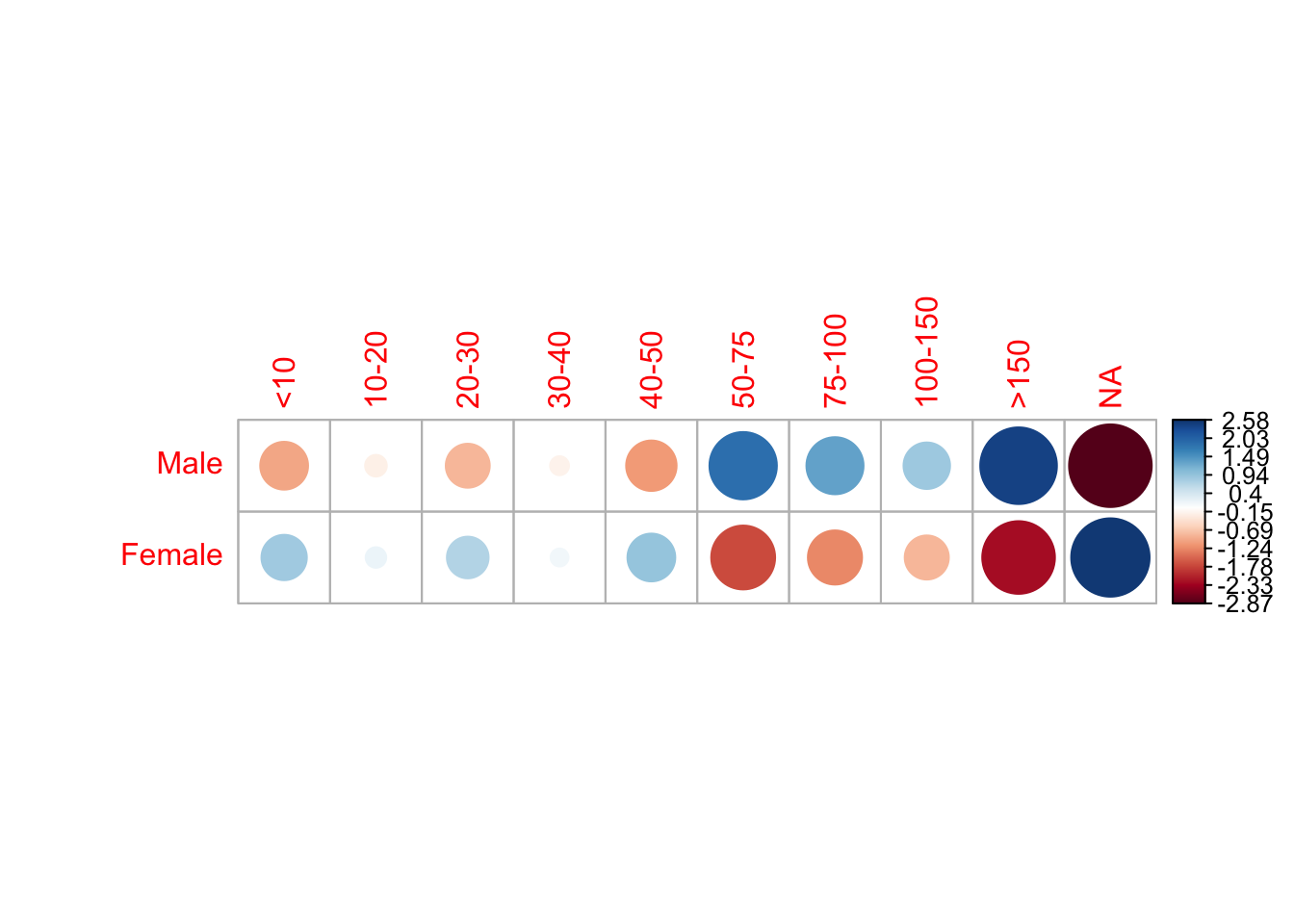
As predicted by our p-value, we can see there is a difference in earnings depending on gender.
#test to see if there is a relationship between
#race and income
test2<-chisq.test(df3$race1_1, df3$income)
## Warning in chisq.test(df3$race1_1, df3$income): Chi-squared approximation
## may be incorrecttest2##
## Pearson's Chi-squared test
##
## data: df3$race1_1 and df3$income
## X-squared = 195.77, df = 36, p-value < 2.2e-16In our qui-squared test for independence to find a relationship between race and income level, we found our p-value to be even smaller than before. We can conclude that there is a stronger dependence between race of a worker and their salary level than gender and salary.
corrplot(test2$residuals, is.corr = F)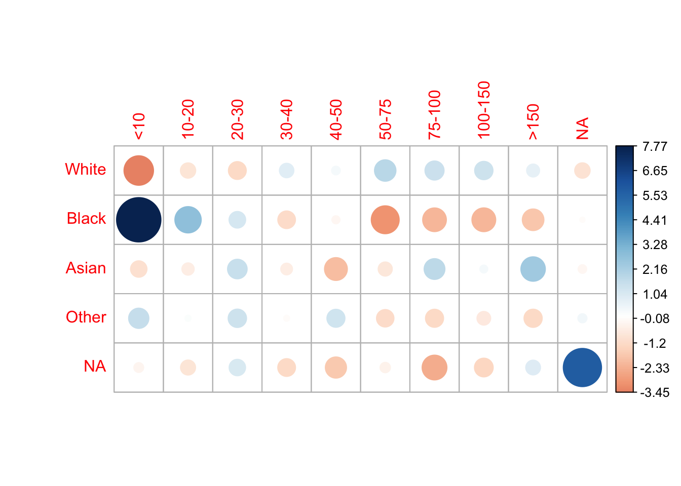
By graphing the relationship between race and income it is easy to see that White and Assian workers have the highest income. In contrast, Black workers by far earn the lowest income.
Eddie’s section
model <- glm(bi_var ~ income, data = df3, family = "binomial")
pander::pander(summary(model))| Estimate | Std. Error | z value | Pr(>|z|) | |
|---|---|---|---|---|
| (Intercept) | 0.2305 | 0.1289 | 1.789 | 0.07369 |
| income10-20 | 0.635 | 0.1786 | 3.556 | 0.0003764 |
| income20-30 | 0.5736 | 0.1772 | 3.238 | 0.001205 |
| income30-40 | 1.08 | 0.1901 | 5.68 | 1.347e-08 |
| income40-50 | 0.8735 | 0.1952 | 4.475 | 7.624e-06 |
| income50-75 | 1.362 | 0.1839 | 7.406 | 1.304e-13 |
| income75-100 | 1.347 | 0.2007 | 6.713 | 1.911e-11 |
| income100-150 | 1.361 | 0.2097 | 6.489 | 8.668e-11 |
| income>150 | 1.163 | 0.2309 | 5.037 | 4.733e-07 |
| incomeNA | 0.6804 | 0.1704 | 3.994 | 6.489e-05 |
(Dispersion parameter for binomial family taken to be 1 )
| Null deviance: | 3329 on 2966 degrees of freedom |
| Residual deviance: | 3233 on 2957 degrees of freedom |
This table separates the “standar error”, “z value” and “p-value” per income level. We found the lowest p-value on the most common income between $50 and $75 thousand per year.